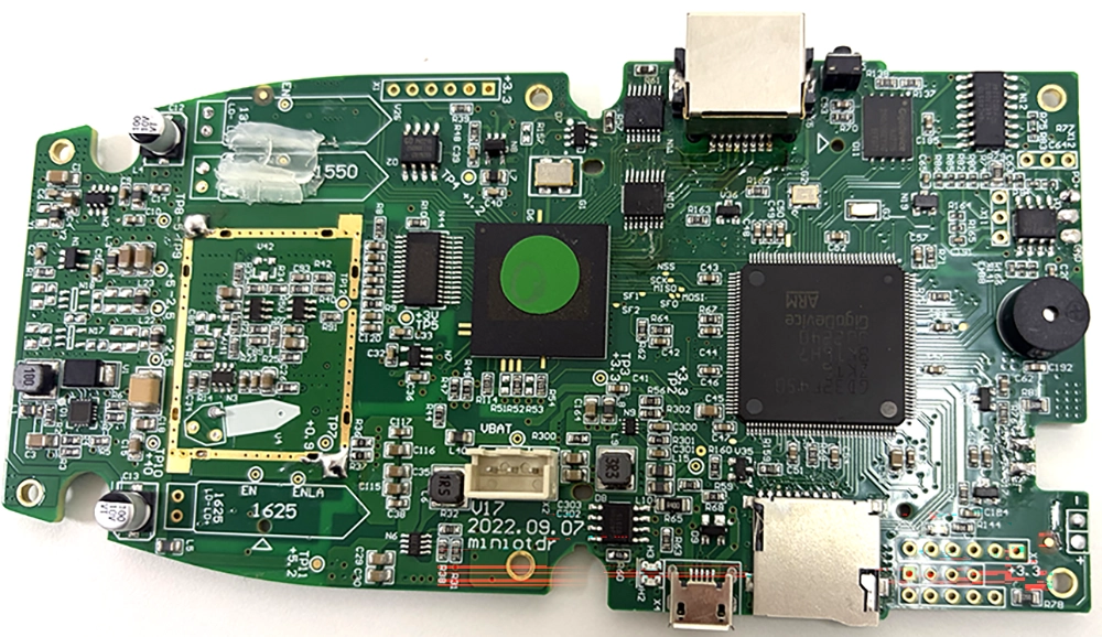
An Optical Time-Domain Reflectometer (OTDR) draws a physical “topology map” of a fiber optic link by injecting optical pulses and analyzing their backscattered and reflected signals. To obtain an accurate test trace, parameters must be precisely configured according to the actual physical characteristics of the link under test. Setting OTDR parameters is essentially a physical trade-off among optical energy injection, Signal-to-Noise Ratio (SNR), and spatial measurement precision.
Optical Waves and Measurement Boundary Settings
The most fundamental parameters determine the physical properties of the test signal and the instrument’s observation window.
Wavelength
The wavelength determines the attenuation and modal characteristics of the optical signal as it travels through the fiber. For single-mode fibers, 1310nm and 1550nm are most commonly used. 1310nm features stronger Rayleigh scattering, offering slightly higher resolution but greater attenuation; 1550nm has lower attenuation, making it suitable for long-distance penetration. In advanced troubleshooting, dual-wavelength testing is often used to diagnose Macro-bending: because longer wavelengths are more sensitive to bending stress, if a significant loss step appears at 1550nm while the 1310nm baseline remains smooth, it can be identified as a physical bend rather than a poor splice. Additionally, 1625nm or 1650nm is dedicated to In-Service/Live Testing; combined with high-isolation filters at the front end, this avoids interfering with active traffic on the network.
Distance Range
The range determines the theoretical end of the X-axis (time/distance axis) for data acquisition, usually set to 1.5 to 2 times the actual fiber length. At the hardware level, the range strictly limits the laser’s Pulse Repetition Rate (PRR). To prevent the far-end echo of the previous pulse from overlapping with the near-end echo of the next pulse, the physical relationship is: . Setting the range too large (increasing ) forces the system to lower the emission frequency, drastically reducing the number of effective pulses averaged per unit time, thereby severely slowing down the SNR improvement.
Distance/Sampling Resolution
Distinct from the “physical spatial resolution” determined by the optical pulse, the distance resolution is the digital granularity dictated by the Analog-to-Digital Converter (ADC) sampling rate. If the ADC sampling frequency is , the resolution is . To accurately reconstruct the edges of ultra-narrow optical pulses without smoothing out steps, the distance resolution must be much smaller than the spatial resolution. However, extreme resolution triggers memory depth disasters. Therefore, high-end OTDRs dynamically balance data density and memory limits via hardware Decimation at large measurement ranges.
The Extreme Game Between Energy and Precision
This set of parameters directly determines “how far” and “how clearly” the device can see, representing the most irreconcilable physical contradiction within an OTDR.
Pulse Width
Pulse width is the Achilles’ heel determining OTDR performance. A longer pulse width (e.g., 10µs) injects massive total energy, yielding an extreme dynamic range (penetration capability); however, it occupies a longer physical space in the fiber (), causing the echoes of adjacent events to overlap, thereby sacrificing spatial resolution. A shorter pulse width (e.g., 5ns) provides ultra-high spatial resolution, but the signal is easily drowned out by thermal noise.
Averaging Time
A single weak Rayleigh signal received by the OTDR is usually buried in white noise; the device must transmit thousands of pulses and perform synchronized time accumulation. According to statistical laws, the SNR improvement is proportional to the square root of the number of averages. Increasing the averaging time from 15 seconds to 3 minutes yields an approximate 2dB to 3dB improvement in dynamic range, but exceeding this time results in diminishing marginal returns.
Event Dead Zone (EDZ) and Attenuation Dead Zone (ADZ)
Dead zones are physical blind spots required for the front-end Avalanche Photodiode (APD) to recover linear response after entering saturation due to strong Fresnel reflections (e.g., fiber end-faces). EDZ is the shortest distance required to distinguish two consecutive reflective events, strictly limited by the pulse width. ADZ is the shortest distance required for the receiver to fully recover from saturation and accurately measure the subsequent Rayleigh baseline. ADZ is always larger than EDZ, heavily testing the active clamping and anti-saturation recovery design of the OTDR’s internal Transimpedance Amplifier (TIA).
Medium Topology and Algorithm Decision Parameters: From Electrical Signals to Physical Truth
Translating time-domain electrical signals accurately into distance-domain physical metrics and determining events rely on fiber dielectric constants and digital thresholds.
Index of Refraction (IOR) and Backscatter Coefficient (BSC)
An OTDR actually measures the time of flight of light; the displayed distance formula is . A minute deviation in the IOR () value will cause severe absolute distance errors in long-haul testing. The BSC affects the absolute power level of the trace. When accurately calculating connector Optical Return Loss (ORL), the BSC must perfectly match the fiber under test, or the calculation will be severely distorted.
Helix Factor
Fibers are wound spirally in loose tubes inside optical cables, meaning the actual optical physical length is always greater than the cable’s outer jacket length. By inputting the helix factor (usually 1% to 2%) into the device, the firmware automatically scales the optical length proportionally to the cable jacket length, enabling precise external fault location.
Event Decision Thresholds
Splice Loss Threshold: Sets the sensitivity lower limit for non-reflective events (splices, macro-bends) (typically 0.05dB for maintenance, 0.01dB for backbone acceptance).
Reflectance Threshold: The red line for identifying Fresnel reflection events relative to baseline abrupt peaks.
End-of-Fiber (EOF) Threshold: The drop-off red line determining the physical end of the link (default is usually 3dB). Once a drop exceeds this value, the algorithm truncates subsequent analysis.
Two-Point Method vs. Five-Point Method (LSA)
After acquiring discrete data points, the DSP must translate complex trace fluctuations into precise “loss” values, relying on underlying mathematical models.
Two-Point Method: Absolute Level Difference
Directly reads the y-coordinates of points and and calculates the difference. This algorithm is extremely sensitive to high-frequency noise; if a sampled point lands exactly in a noise trough, the error is magnified. It is strictly prohibited for micro-measurement of individual splices and is only applicable for evaluating the macroscopic total attenuation of fiber sections kilometers long.
Five-Point Method / Least Squares Approximation (LSA): Noise-Immune Linear Regression
This is the industry gold standard for measuring splice/connector insertion loss. Using 5 markers, the algorithm frames two pure Rayleigh scattering intervals before the event and after the dead zone tail. The DSP extracts hundreds of data points from these two segments to execute linear regression (LSA), fits two optimal straight lines, and mathematically projects them toward the “event center.” The final loss is the difference in the intercepts of the two ideal lines at the center. Algorithmic Value: It mathematically completely strips away the “dead zone tail effect” caused by hardware AFE saturation recovery. When processing splices of fibers with different mode field diameters, it can also accurately reveal the physically non-existent “Gainer” (pseudo-gain) phenomenon.
Special Parameter Scheduling for Complex PON Networks
In Passive Optical Networks (PON), 1:N optical splitters create massive step-like cliffs ranging from 10dB to 22dB, rendering conventional parameter logic completely ineffective.
Reconstructing the EOF Threshold
A standard 3dB EOF will misidentify a splitter as a fiber break. PON modes must forcefully raise the EOF to 25dB or higher, or disable the parameter entirely, relying instead on the absolute noise floor beneath the reflection peak to determine the link’s end.
Multi-Pulse Stitching Algorithm
A single pulse width cannot cater to testing both before and after a splitter. High-end smart firmware automatically schedules in the background: ultra-narrow pulses for near-end fine mapping (measuring connectors); medium pulses for outlining macroscopic steps; and ultra-wide pulses to forcefully penetrate the splitter using massive energy. Subsequently, the DSP performs weighted data fusion and stitching based on SNR crossing points to generate a virtual trace boasting both high resolution and high penetration.
Extreme Averaging and Dynamic VGA Control
The far-end signal after penetrating a splitter often drops below -60dBm, requiring the averaging time to be extended to 3 to 5 minutes. Simultaneously, based on the time of flight, the firmware dynamically increases the front-end Variable Gain Amplifier (VGA) the instant the pulse passes through the splitter, ensuring the front section does not overload and the rear section is not missed.
sor Format and Binary Encapsulation
Hardware acquisition and DSP computation results are ultimately encapsulated into a compact binary file conforming to the Telcordia specification, the .sor (Standard OTDR Record), for cross-platform offline analysis.
Structured Block Design
The file is compactly composed of a Map Block (directory addressing), General Parameters, Fixed Parameters (saving pulse width, IOR, BSC, etc., as reconstruction baselines), Data Points (raw waveform sequence), and Key Events (the final event table identified by the firmware).
Quantization and Scaling Factor
To compress file size, massive arrays of optical power points do not use floating-point numbers. Instead, they use “fixed-point integers + scaling factors” (e.g., 12.345dB scaled and stored as the integer 12345). Under high dynamic testing, high-end OTDRs must dynamically declare a switch to 32-bit encoding in the protocol header to prevent integer overflow.
Proprietary Blocks (Hidden Extensions)
Manufacturers can covertly inject custom blocks into the file. R&D teams can encapsulate underlying sub-traces from multi-pulse composite tests, macro-bending diagnostic metadata, and even low-level AFE temperature and bias voltage logs. These data remain transparent and compatible with third-party standard viewers, yet provide the original manufacturer with an irreplaceable data foundation for remote troubleshooting and AI training.
FirstFiber Technologies provides professional technical support and OTDR customization services (covering core algorithms, hardware architecture design, and testing solutions for special conditions). For technical consultations or customized requirements, please feel free to contact us.